Introduction guide

Introduction guide#

This guide was almost completely adapted from the great NumPy: the absolute basics for beginners tutorial. You can also check out this other guide with more illustrations.

NumPy (Numerical Python) is an open source Python library that’s widely used in science and engineering. The NumPy library contains multidimensional array data structures, such as the homogeneous, N-dimensional ndarray, and a large library of functions that operate efficiently on these data structures.

How to import NumPy#

After installing NumPy, it may be imported into Python code like:

import numpy as np

This widespread convention allows access to NumPy features with a short, recognizable prefix (np.) while distinguishing NumPy features from others that have the same name.

Why use NumPy?#

Python lists are excellent, general-purpose containers. They can be “heterogeneous”, meaning that they can contain elements of a variety of types, and they are quite fast when used to perform individual operations on a handful of elements.

Depending on the characteristics of the data and the types of operations that need to be performed, other containers may be more appropriate; by exploiting these characteristics, we can improve speed, reduce memory consumption, and offer a high-level syntax for performing a variety of common processing tasks. NumPy shines when there are large quantities of “homogeneous” (same-type) data to be processed on the CPU.

To illustrate the performance boost NumPy can offer, we perform the same operations, first in pure Python, then using NumPy, and time both of them:

%%time
li = [i for i in range(1000000)]
list_sum = sum(li)

CPU times: user 89.3 ms, sys: 97 ms, total: 186 ms
Wall time: 51 ms

%%time
arr = np.arange(1000000)
arr_sum = np.sum(arr)

CPU times: user 0 ns, sys: 1.7 ms, total: 1.7 ms
Wall time: 1.7 ms

Tip

Note the use of the %%time cell magic, it is very useful to compare the performance of two pieces of code!

What is an “array”?#

In computer programming, an array is a structure for storing and retrieving data. We often talk about an array as if it were a grid in space, with each cell storing one element of the data. For instance, if each element of the data were a number, we might visualize a “one-dimensional” array like a list:

\[\begin{split}\begin{aligned} \begin{array}{|c||c|c|c|} \hline 1 & 5 & 2 & 0 \\ \hline \end{array} \end{aligned}\end{split}\]

A two-dimensional array would be like a table:

\[\begin{split}\begin{aligned} \begin{array}{|c||c|c|c|} \hline 1 & 5 & 2 & 0 \\ \hline 8 & 3 & 6 & 1 \\ \hline 1 & 7 & 2 & 9 \\ \hline \end{array} \end{aligned}\end{split}\]

A three-dimensional array would be like a set of tables, perhaps stacked as though they were printed on separate pages. In NumPy, this idea is generalized to an arbitrary number of dimensions, and so the fundamental array class is called ndarray: it represents an “N-dimensional array”.

Most NumPy arrays have some restrictions. For instance:

All elements of the array must be of the same type of data.
Once created, the total size of the array can’t change.
The shape must be “rectangular”, not “jagged”; e.g., each row of a two-dimensional array must have the same number of columns.

When these conditions are met, NumPy exploits these characteristics to make the array faster, more memory efficient, and more convenient to use than less restrictive data structures.

For the remainder of this document, we will use the word “array” to refer to an instance of ndarray.

Array fundamentals#

One way to initialize an array is using a Python sequence, such as a list. For example:

a = np.array([1, 2, 3, 4, 5, 6])
a

array([1, 2, 3, 4, 5, 6])

Elements of an array can be accessed in various ways. For instance, we can access an individual element of this array as we would access an element in the original list: using the integer index of the element within square brackets.

a[0]

Note

As with built-in Python sequences, NumPy arrays are “0-indexed”: the first element of the array is accessed using index 0, not 1.

Like the original list, the array is mutable.

a[0] = 10
a

array([10,  2,  3,  4,  5,  6])

Also like the original list, Python slice notation can be used for indexing.

a[:3]

array([10,  2,  3])

One major difference is that slice indexing of a list copies the elements into a new list, but slicing an array returns a view: an object that refers to the data in the original array. The original array can be mutated using the view.

b = a[3:]
b

array([4, 5, 6])

Question

Given that information, try to guess the output of the cell below before running it.

b[0] = 40
a

Two- and higher-dimensional arrays can be initialized from nested Python sequences:

a = np.array([[1, 2, 3, 4], [5, 6, 7, 8], [9, 10, 11, 12]])
a

array([[ 1,  2,  3,  4],
       [ 5,  6,  7,  8],
       [ 9, 10, 11, 12]])

In NumPy, a dimension of an array is sometimes referred to as an “axis”. This terminology may be useful to disambiguate between the dimensionality of an array and the dimensionality of the data represented by the array. For instance, the array a could represent three points, each lying within a four-dimensional space, but a has only two “axes”.

Another difference between an array and a list of lists is that an element of the array can be accessed by specifying the index along each axis within a single set of square brackets, separated by commas. For instance, the element 8 is in row 1 and column 3:

a[1, 3]

Note

You might hear of a 0-D (zero-dimensional) array referred to as a “scalar”, a 1-D (one-dimensional) array as a “vector”, a 2-D (two-dimensional) array as a “matrix”, or an N-D (N-dimensional, where “N” is typically an integer greater than 2) array as a “tensor”. For clarity, it is best to avoid the mathematical terms when referring to an array because the mathematical objects with these names behave differently than arrays (e.g. “matrix” multiplication is fundamentally different from “array” multiplication), and there are other objects in the scientific Python ecosystem that have these names (e.g. the fundamental data structure of PyTorch is the “tensor”).

Array attributes#

The number of dimensions of an array is contained in the ndim attribute.

a.ndim

The shape of an array is a tuple of non-negative integers that specify the number of elements along each dimension.

a.shape

(3, 4)

The fixed, total number of elements in array is contained in the size attribute.

a.size

Arrays are typically “homogeneous”, meaning that they contain elements of only one “data type”. The data type is recorded in the dtype attribute.

a.dtype

dtype('int64')

How to create a basic array#

Besides creating an array from a sequence of elements, you can easily create an array filled with 0’s:

np.zeros(2)

array([0., 0.])

Or an array filled with 1’s:

np.ones(2)

array([1., 1.])

While the default data type is floating point (np.float64), you can explicitly specify which data type you want using the dtype keyword. :

x = np.ones(2, dtype=np.int64)
x

array([1, 1])

You can also create an array filled with a specific value, using np.full():

np.full((2, 3), 42)

array([[42, 42, 42],
       [42, 42, 42]])

You can also create an array with a range of elements:

np.arange(4)

array([0, 1, 2, 3])

And even an array that contains a range of evenly spaced intervals. To do this, you will specify that the generated numbers should be between a first number and a last one (excluded), and spaced by a step size. :

np.arange(2, 9, 2)

array([2, 4, 6, 8])

Question

How would you create the equivalent list, in a single line?

[2, 4, 6, 8]

You can also use np.linspace() to create an array with num values spaced linearly in a specified interval:

np.linspace(0, 10, num=5)

array([ 0. ,  2.5,  5. ,  7.5, 10. ])

Basic array operations#

Once you’ve created your arrays, you can start to work with them. Let’s say, for example, that you’ve created two arrays, one called “data” and one called “ones”

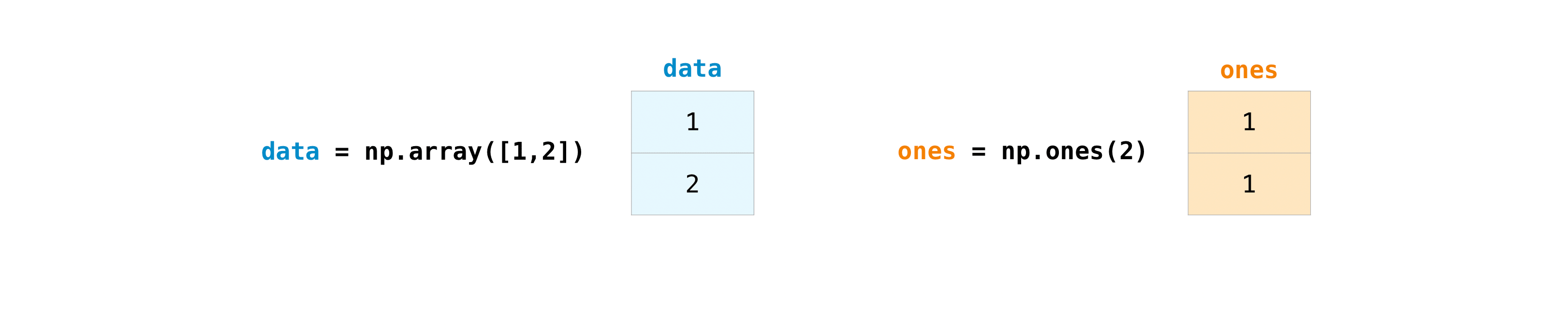
You can add the arrays together with the plus sign.

data = np.array([1, 2])
ones = np.ones(2, dtype=int)
data + ones

array([2, 3])

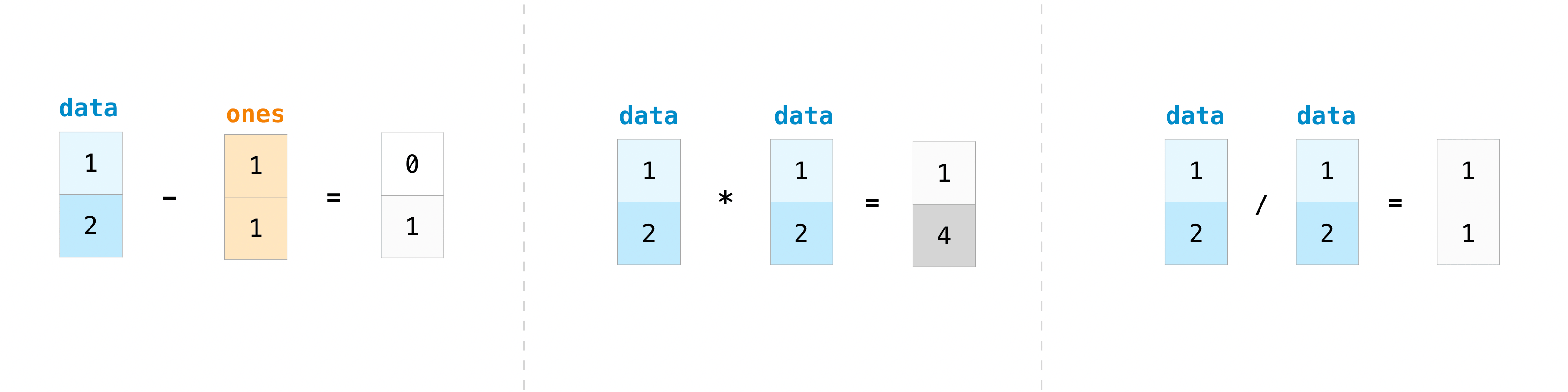
You can, of course, do more than just addition!

data - ones, data * data, data / data

(array([0, 1]), array([1, 4]), array([1., 1.]))

How to create an array from existing data#

You can easily create a new array from a section of an existing array.

Let’s say you have this array:

a = np.array([1, 2, 3, 4, 5, 6, 7, 8, 9, 10])

You can concatenate it to another, to add new entries:

np.concatenate([a, np.array([11, 12])])

array([ 1,  2,  3,  4,  5,  6,  7,  8,  9, 10, 11, 12])

You can stack two existing arrays, both vertically and horizontally. Let’s say you have two arrays, a1 and a2:

a1 = np.array(
    [
        [1, 1],
        [2, 2],
    ]
)
a2 = np.array(
    [
        [3, 3],
        [4, 4],
    ]
)

You can stack them vertically with vstack:

np.vstack([a1, a2])

array([[1, 1],
       [2, 2],
       [3, 3],
       [4, 4]])

or, equivalently, concatenating them together along the rows, by passing axis=0 to np.concatenate():

np.concatenate([a1, a2], axis=0)

array([[1, 1],
       [2, 2],
       [3, 3],
       [4, 4]])

Or stack them horizontally with hstack:

np.hstack([a1, a2])

array([[1, 1, 3, 3],
       [2, 2, 4, 4]])

or, again, equivalently, concatenating them together along the columns, by passing axis=1 to np.concatenate():

np.concatenate([a1, a2], axis=1)

array([[1, 1, 3, 3],
       [2, 2, 4, 4]])

Transposing and reshaping a matrix#

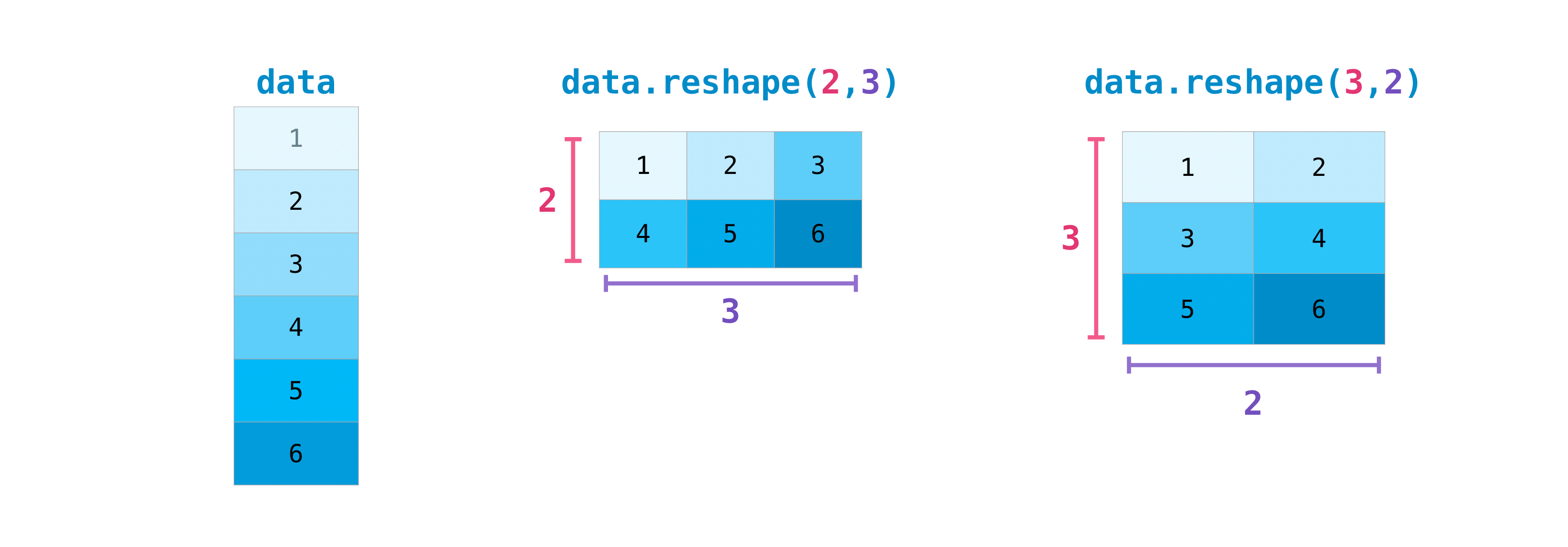
data = np.arange(1, 7)

You may also need to switch the dimensions of a matrix. This can happen when, for example, you have a model that expects a certain input shape that is different from your dataset. This is where the reshape method can be useful. You simply need to pass in the new dimensions that you want for the matrix. :

data = data.reshape((2, 3))
data

array([[1, 2, 3],
       [4, 5, 6]])

data = data.reshape((3, 2))
data

array([[1, 2],
       [3, 4],
       [5, 6]])

You can transpose your array with arr.transpose(). :

data.transpose()

array([[1, 3, 5],
       [2, 4, 6]])

You can also use data.T:

data.T

array([[1, 3, 5],
       [2, 4, 6]])

Note that this is different from data.reshape(data.shape[::-1]): the latter keeps the order of the elements reading from left to right and top to bottom, while transposing transforms rows into columns, thus switching the two dimensions.

Question

Is the following code going to work? Why, or why not?

data.reshape((3,3))

Answer

No, because data has a shape (3, 2), so 3 * 2 = 6 elements, while the shape (3, 3) would require 3 * 3 = 9 elements

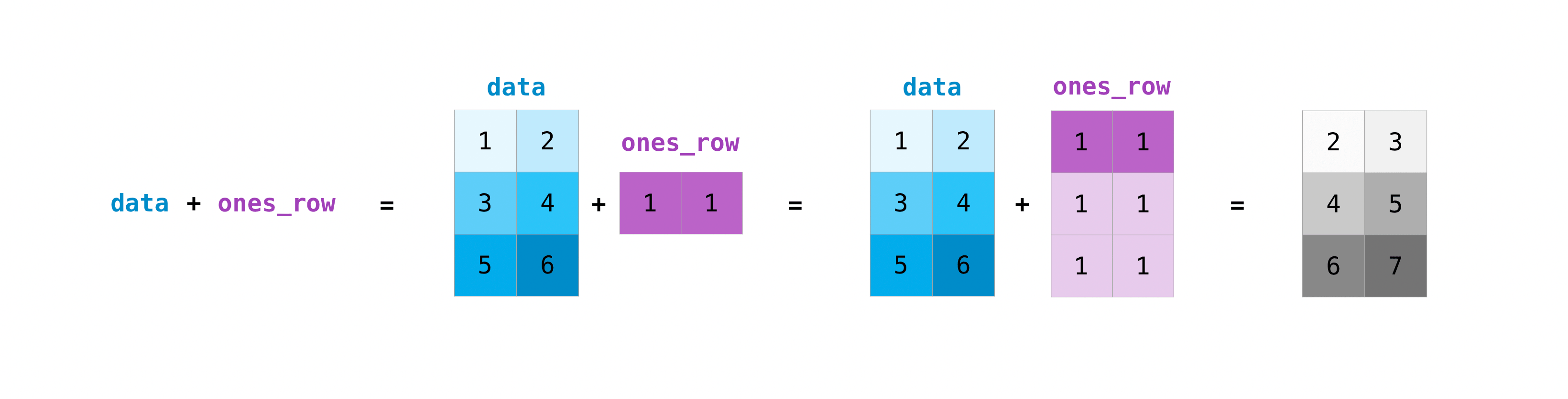
Broadcasting#

There are times when you might want to carry out an operation between an array and a single number (also called an operation between a vector and a scalar) or between arrays of two different sizes. For example, your array (we’ll call it “data”) might contain information about distance in miles but you want to convert the information to kilometers. You can perform this operation with:

data = np.array([1.0, 2.0])
data * 1.6

array([1.6, 3.2])

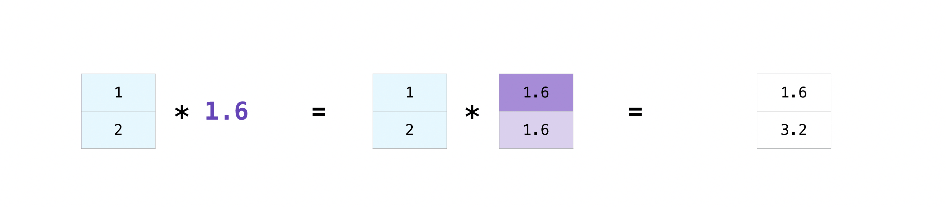
NumPy understands that the multiplication should happen with each cell. That concept is called broadcasting. Broadcasting is a mechanism that allows NumPy to perform operations on arrays of different shapes. The dimensions of your array must be compatible, for example, when the dimensions of both arrays are equal or when one of them is 1. If the dimensions are not compatible, you will get a ValueError.

This works with scalars, but not only! For matrices, you can do these arithmetic operations on matrices of different sizes, but only if one matrix has only one column or one row. In this case, NumPy will use its broadcast rules for the operation. :

data = np.array([[1, 2], [3, 4], [5, 6]])
ones_row = np.array([[1, 1]])
data + ones_row

array([[2, 3],
       [4, 5],
       [6, 7]])

Question

What would be the result of the following sum?

range_col = np.arange(3).reshape((3, 1))
data + range_col

Selecting part of an array#

By index#

You can index and slice NumPy arrays in the same ways you can slice Python lists. :

data = np.array([1, 2, 3])
data[1]

data[0:2]

array([1, 2])

data[1:]

array([2, 3])

data[-2:]

array([2, 3])

You can visualize it this way:

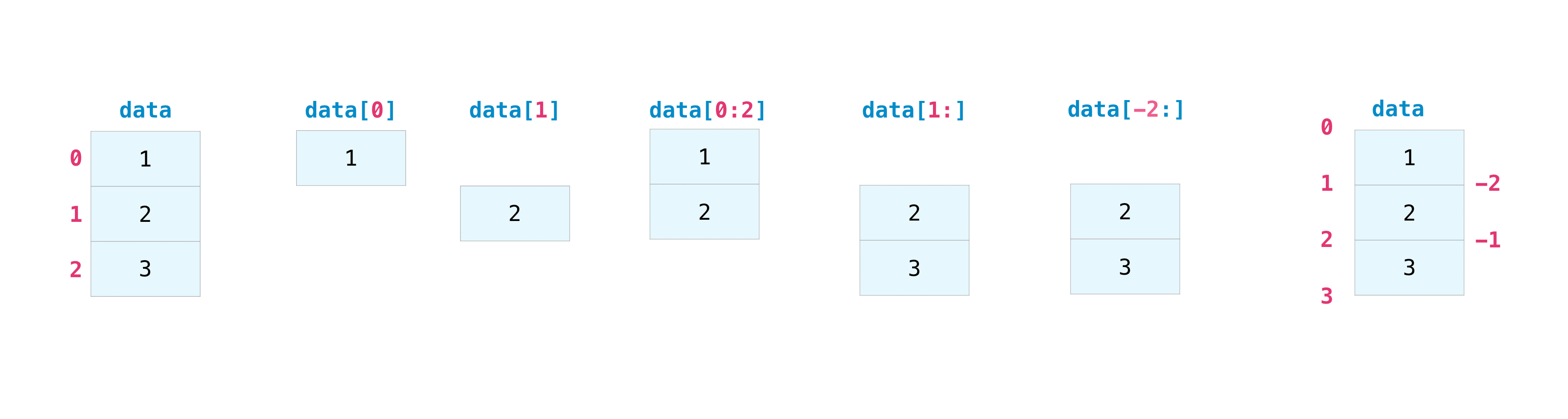
You may want to take a section of your array or specific array elements to use in further analysis or additional operations. To do that, you’ll need to subset, slice, and/or index your arrays.

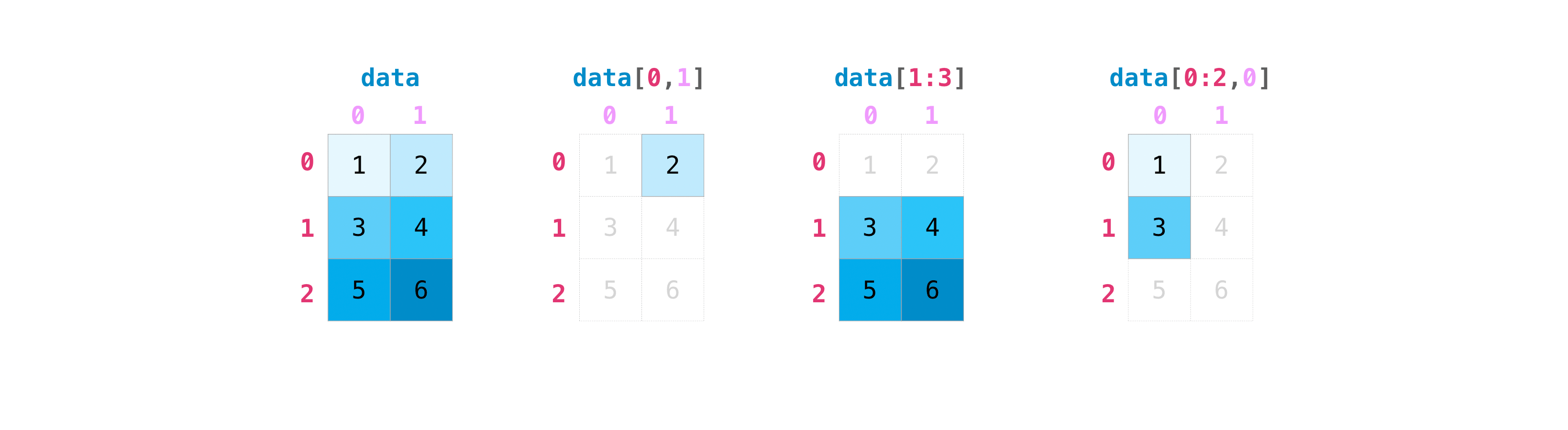
Same goes in more than one dimension, you may specify an index or slice along each dimension.

data = np.array([[1, 2], [3, 4], [5, 6]])

Like for instance, to select a single element:

data[0, 1]

Slicing over the rows only:

data[1:3]

array([[3, 4],
       [5, 6]])

Or taking a single column, and a slice of rows:

data[0:2, 0]

array([1, 3])

By array of indices#

You may also provide arrays of indices to select:

data[np.array([1, 2])]

array([[3, 4],
       [5, 6]])

Which, as expected, returns the second and third rows.

Question

Since data[1:3] is equivalent to data[1:3, 0:2], what would you expect the following to return?

data[np.arange(1, 3), np.arange(0, 2)]

Probably not what you expected, uh? Why so? To answer that, let’s see what happens if we write what we’d naively think the equivalent of data[0:3, 0:2] to be:

data[np.arange(0, 3), np.arange(0, 2)]

---------------------------------------------------------------------------
IndexError                                Traceback (most recent call last)
Cell In[52], line 1
----> 1 data[np.arange(0, 3), np.arange(0, 2)]

IndexError: shape mismatch: indexing arrays could not be broadcast together with shapes (3,) (2,) 

This does not just have an unexpected behaviour, it doesn’t even work! But what’s the problem? Inspecting the error, we see that the source of the problem is a broadcasting error. And when can a broadcasting error come up? This is a hard one but you may have guessed it: when we… try to broadcast.

In fact, NumPy first takes the two arrays we pass it, and tries to broadcast them to a common shape, as can for instance be done successfully for the two following arrays:

rows = np.arange(1, 3)
cols = np.array([[0, 1], [0, 1]])
np.broadcast_arrays(rows, cols)

[array([[1, 2],
        [1, 2]]),
 array([[0, 1],
        [0, 1]])]

Then, since they are broadcastable, the following does work:

data[rows, cols]

array([[3, 6],
       [3, 6]])

As you can see, the result has the same shape as each output of the broadcasting. So, actually, in each broadcasted input, each element corresponds to the index to select from data along the dimension they represent. So for instance, the top left element will be taken from the second row (index=1) and the first column (index=0).

Question

So what happened when we ran data[np.arange(1, 3), np.arange(0, 2)] above?

Answer

This is a simpler example than what we just saw: here the broadcasting doesn’t do anything, since the two input arrays have the same shape, equal to (2,). So this just created an array of shape (2,), in which the first element is taken from data[1, 0] (= 3), and the second from data[2, 1] (= 6).

By condition#

If you want to select values from your array that fulfill certain conditions, it’s straightforward with NumPy.

For example, if you start with this array:

a = np.array([[1, 2, 3, 4], [5, 6, 7, 8], [9, 10, 11, 12]])

If you want to know where this array has values inferior to 5, you can create the following variable:

five_up = (a >= 5)
five_up

array([[False, False, False, False],
       [ True,  True,  True,  True],
       [ True,  True,  True,  True]])

Showing you with True values where the condition is fulfilled, and False where it is not. The variable five_up is what is known as a boolean mask: you can use it to mask part of an array to select only part of it, but also to modify part of it! You can easily print all of the values in the array that are superior to 5 like so:

a[five_up]

array([ 5,  6,  7,  8,  9, 10, 11, 12])

or directly, without assigning the variable five_up:

a[a >= 5]

array([ 5,  6,  7,  8,  9, 10, 11, 12])

Not only that, we can also build more complex expressions by using

& symbol as the logical conjunction and
| (pipe character) as the logical conjunction or

a[(a > 2) & (a < 11)] = 0
a

array([[ 1,  2,  0,  0],
       [ 0,  0,  0,  0],
       [ 0,  0, 11, 12]])

Warning

Remember the round parenthesis among the various expressions!

Exercise: try to rewrite the expressions above by ‘forgetting’ the round parenthesis in the various components (left/right/both) and see what happens. Do you obtain errors or unexpected results?

a = np.array([[1, 2, 3, 4], [5, 6, 7, 8], [9, 10, 11, 12]])

print(a[(a > 3) & a < 6])
print(a[a > 3 & (a < 6)])
print(a[a > 3 & a < 6])

You can also use np.nonzero() to select elements or indices from an array.

Starting with this array:

a = np.array([[1, 2, 3, 4], [5, 6, 7, 8], [9, 10, 11, 12]])

You can use np.nonzero() to print the indices of elements that are, for example, less than 5:

b = np.nonzero(a < 5)
b

(array([0, 0, 0, 0]), array([0, 1, 2, 3]))

In this example, a tuple of arrays was returned: one for each dimension. The first array represents the row indices where these values are found, and the second array represents the column indices where the values are found.

If you want to generate a list of coordinates where the elements exist, you can zip the arrays, iterate over the list of coordinates, and print them. For example:

list_of_coordinates = list(zip(b[0], b[1]))
for row, col in list_of_coordinates:
    print((row, col))

(0, 0)
(0, 1)
(0, 2)
(0, 3)

You can also use np.nonzero() to print the elements in an array that are less than 5 with:

print(a[b])

[1 2 3 4]

If the element you’re looking for doesn’t exist in the array, then the returned array of indices will be empty. For example:

not_there = np.nonzero(a == 42)
print(not_there)

(array([], dtype=int64), array([], dtype=int64))

Exercise: modify the arrays floored1 and floored2 so that their minimum value is 5, in two ways:

using a boolean mask directly
using np.nonzero()

floored1 = a.copy()
floored2 = a.copy()

array([[ 5,  5,  5,  5],
       [ 5,  6,  7,  8],
       [ 9, 10, 11, 12]])

array([[ 5,  5,  5,  5],
       [ 5,  6,  7,  8],
       [ 9, 10, 11, 12]])

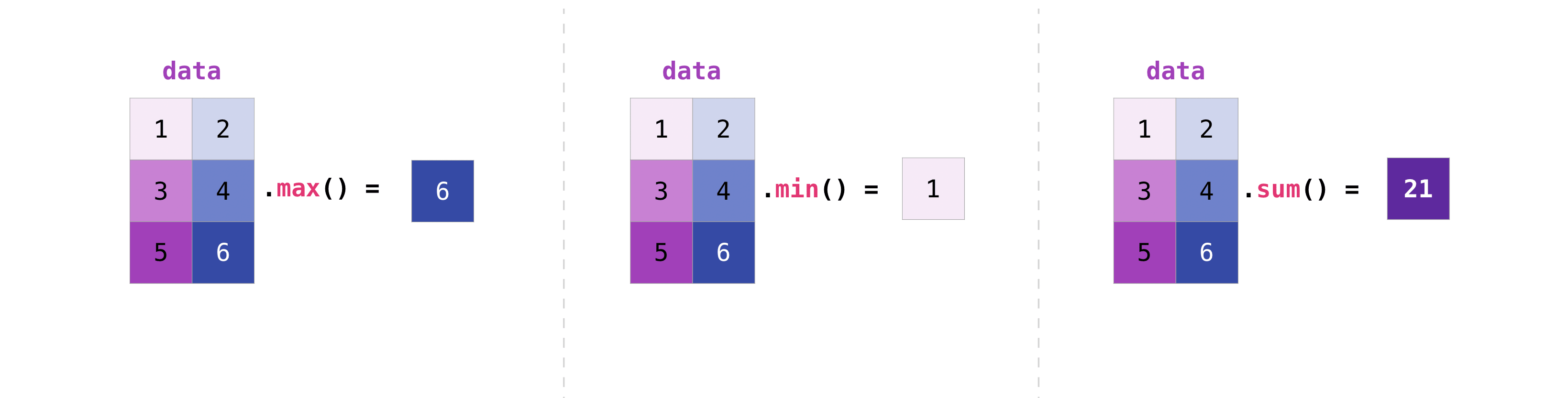
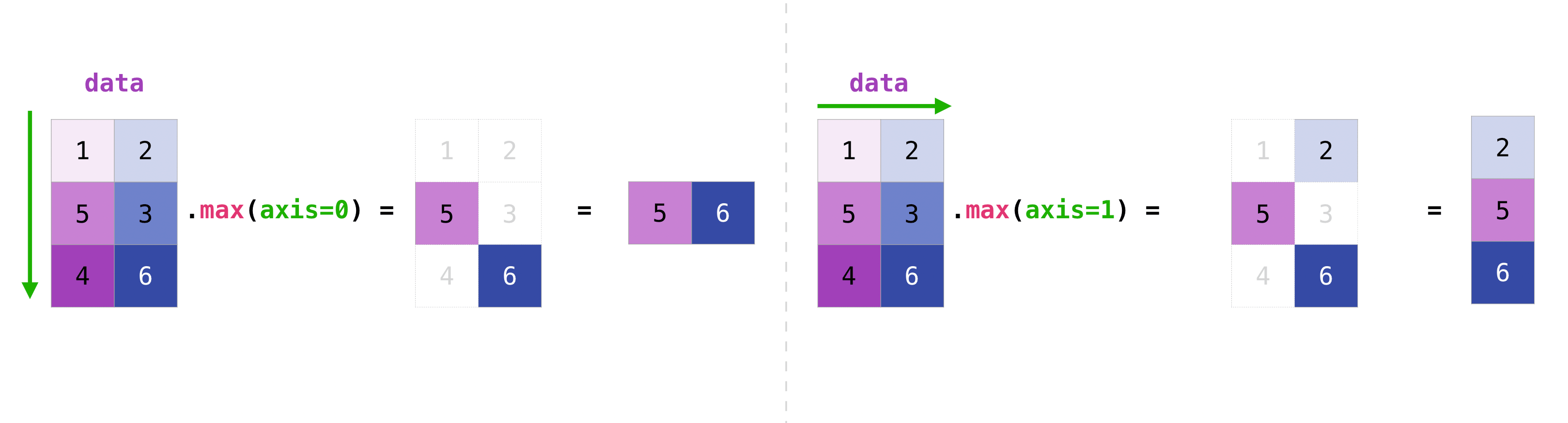
Array aggregation#

NumPy also performs aggregation functions, such as min, max, sum, mean to get the average, prod to get the result of multiplying the elements together, std to get the standard deviation, and more. :

data = np.array([[1, 2], [5, 3], [4, 6]])
data

array([[1, 2],
       [5, 3],
       [4, 6]])

data.max(), data.min(), data.sum()

(6, 1, 21)

As you can see, by default, every NumPy aggregation function will return the aggregate of the entire array. But it’s very common to want to aggregate along a row or column. For that, you need to say explicitly over which axis you wish your aggregation to run.

For instance, you can get the maximum over the axis of rows with:

data.max(axis=0)

array([5, 6])

You can get it over the axis of columns with:

data.max(axis=1)

array([2, 5, 6])

Working with mathematical formulas#

The ease of implementing mathematical formulas that work on arrays is one of the things that make NumPy so widely used in the scientific Python community.

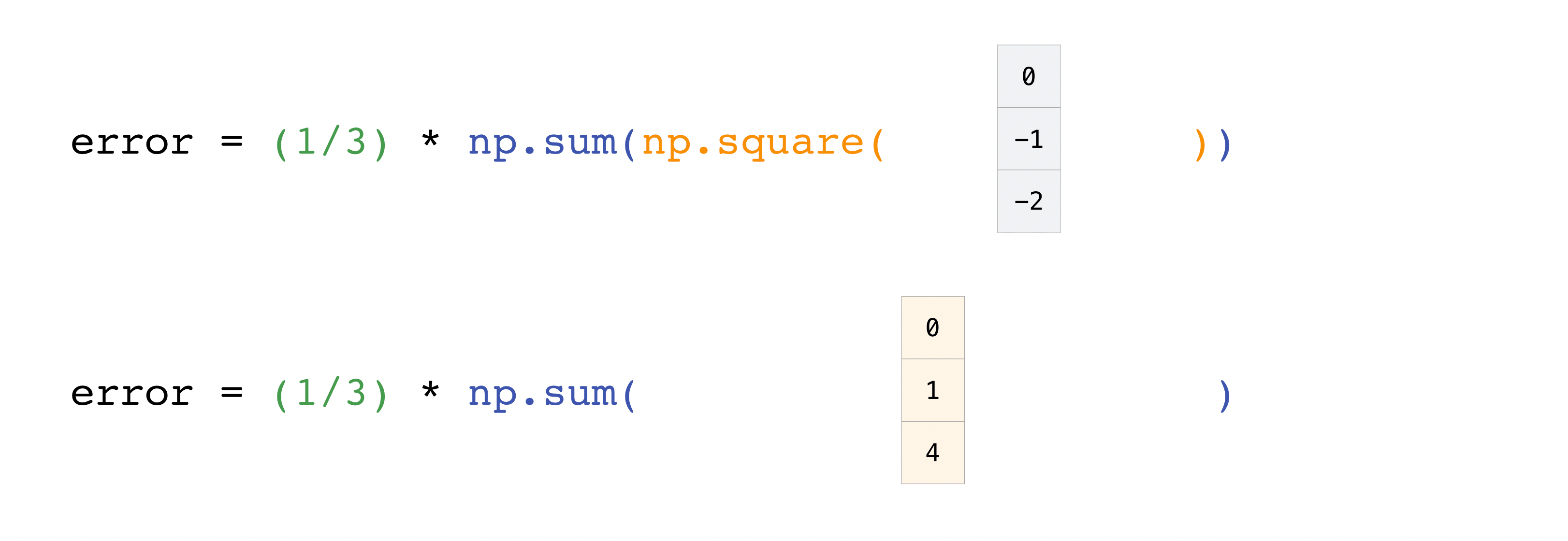
For example, this is the mean square error formula (a central formula used in supervised machine learning models that deal with regression):

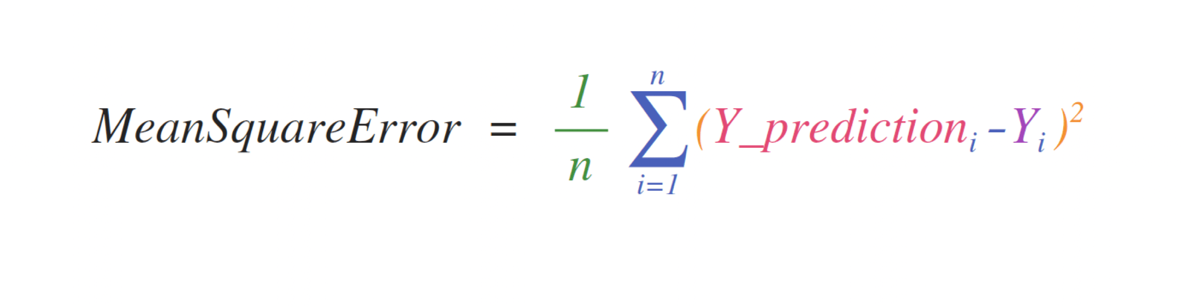
Implementing this formula is simple and straightforward in NumPy:

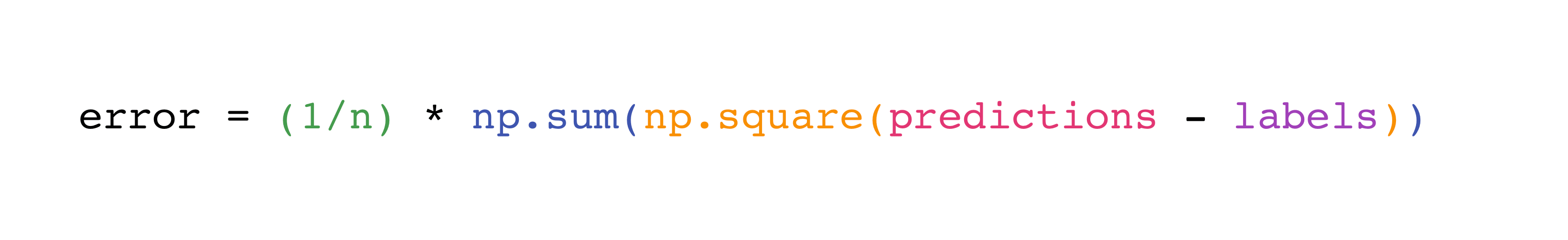
What makes this work so well is that predictions and labels can contain one or a thousand values. They only need to be the same size.

You can visualize it this way:

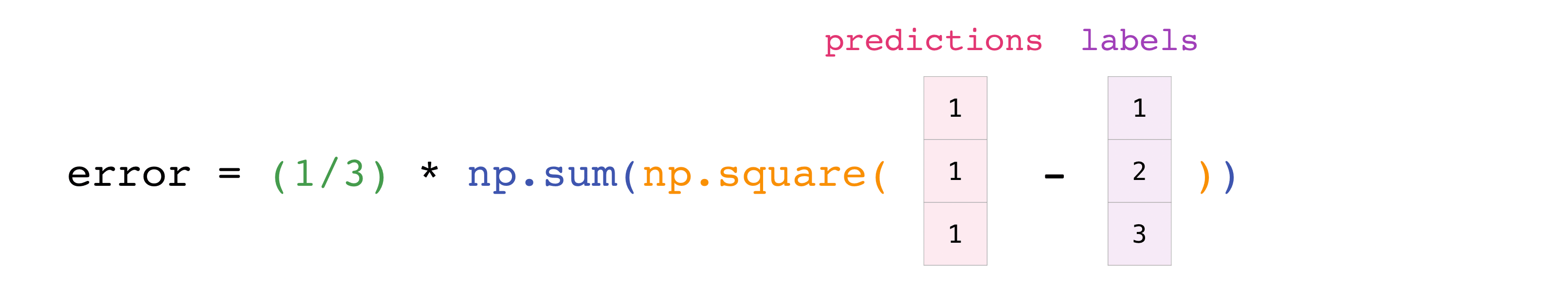
In this example, both the predictions and labels vectors contain three values, meaning n has a value of three. After we carry out subtractions the values in the vector are squared. Then NumPy sums the values, and your result is the error value for that prediction and a score for the quality of the model.

NaNs and infinites#

Some operations may lead to situations that are not mathematically defined, or that yield infinite results. Let’s have a brief overview of these two situations.

NaNs#

A NaN is Not a Number, that you can get from NumPy simply as:

np.nan

nan

But it is actually considered a float:

type(np.nan)

float

So it’s a float number that is not a number, and more interesting even, that’s not equal to itself:

np.nan == np.nan

False

In reality, np.nan is not equal to anything, and further, any test that involves it on one side or the other of the test will return False. So for instance, as shown below, it is neither positive, nor negative or equal to 0:

not (np.nan > 0) and not (np.nan < 0) and not (np.nan == 0)

True

Further, (almost) any operation involving it will return np.nan as well:

0 * np.nan

nan

But so, what’s the point of having this number? To answer that, let’s talk a bit about maths.

In maths, some functions are not defined for a certain range of values. For instance, the logarithm log(x) has the following behaviour:

\(x < 0\): not defined
\(x = 0\): tends to minus infinity
\(x > 0\): defined

log function

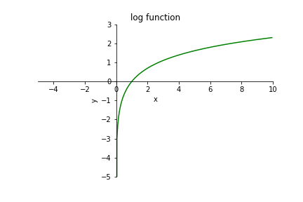
So to define a log function in NumPy, what do we do when users pass values that are inferior to 0? One option could have been to raise an error. But if one single negative value is passed in a large array, this would discard the whole result of some computations. So, instead, the standard defining floating point numbers created this particular float to represent an undefined result. Therefore, the log function in NumPy returns nan when passed a negative number:

np.log([-1, 2, 3])

/tmp/ipykernel_2523/2474035747.py:1: RuntimeWarning: invalid value encountered in log
  np.log([-1, 2, 3])

array([       nan, 0.69314718, 1.09861229])

and raises a warning, instead of an error. Thankfully, a special function np.isnan() is provided to detect their presence:

np.isnan(np.log([-1, 2, 3]))

/tmp/ipykernel_2523/1668739231.py:1: RuntimeWarning: invalid value encountered in log
  np.isnan(np.log([-1, 2, 3]))

array([ True, False, False])

Infinite#

More straightforward are infinite numbers. Since they are infinitely large, it’s not safe to represent the infinite by an arbitrarily large number, so, instead, a special floating-point number is used to represent it:

np.log(0)

/tmp/ipykernel_2523/2933082444.py:1: RuntimeWarning: divide by zero encountered in log
  np.log(0)

-inf

Which, similarly to nan, can be identified with:

np.isinf(np.log([0, 1, 2]))

/tmp/ipykernel_2523/1630574277.py:1: RuntimeWarning: divide by zero encountered in log
  np.isinf(np.log([0, 1, 2]))

array([ True, False, False])

What to do with them?#

So, given an array which might have values leading to these behaviours, what do we do? Suppose we have the following example array:

arr = np.array([-1, 0, 1, 2])

And a function with some undefined domain, like log.

Either you filter the array passed to np.log(), ensuring that whatever you pass it is within the range of values for which the function is properly defined:

np.log(arr[arr > 0])

array([0.        , 0.69314718])

Or you filter values a posteriori:

res = np.log(arr)
res[~np.isnan(res) & (~np.isinf(res))]

/tmp/ipykernel_2523/3078605770.py:1: RuntimeWarning: divide by zero encountered in log
  res = np.log(arr)
/tmp/ipykernel_2523/3078605770.py:1: RuntimeWarning: invalid value encountered in log
  res = np.log(arr)

array([0.        , 0.69314718])

Note that in this example, the latter is more cumbersome. However, sometimes you might get an array with NaNs from another source, or they might be used to represent missing data, so it’s good to be able to handle them.

How to save and load NumPy objects#

You will, at some point, want to save your arrays to disk and load them back without having to re-run the code. Fortunately, there are several ways to save and load objects with NumPy. The ndarray objects can be saved to and loaded from the disk files with loadtxt and savetxt functions that handle normal text files, load and save functions that handle NumPy binary files with a .npy file extension, and a savez function that handles NumPy files with a .npz file extension.

Note

The .npy and .npz files store data, shape, dtype, and other information required to reconstruct the ndarray in a way that allows the array to be correctly retrieved, even when the file is on another machine with different architecture.

Here, we will only cover loadtxt and savetxt though, as they’ll also allow us to refresh your memory on reading and writing text files.

You can save a NumPy array as a plain text file like a .csv or .txt file with np.savetxt.

For example, if you create this array:

csv_arr = np.array([1, 2, 3, 4, 5, 6, 7, 8])

You can easily save it as a .csv file with the name “new_file.csv” like this:

np.savetxt('new_file.csv', csv_arr)

You can quickly and easily load your saved text file using loadtxt():

np.loadtxt('new_file.csv')

array([1., 2., 3., 4., 5., 6., 7., 8.])

The savetxt() and loadtxt() functions accept additional optional parameters such as header, footer, and delimiter.

Image credits: Jay Alammar https://jalammar.github.io/

Introduction guide

Contents

Introduction guide#

How to import NumPy#

Why use NumPy?#

What is an “array”?#

Array fundamentals#

Array attributes#

How to create a basic array#

Basic array operations#

How to create an array from existing data#

Transposing and reshaping a matrix#

Broadcasting#

Selecting part of an array#

By index#

By array of indices#

By condition#

Array aggregation#

Working with mathematical formulas#

NaNs and infinites#

NaNs#

Infinite#

What to do with them?#

How to save and load NumPy objects#