Advanced stuff#
Let’s see how to do more advanced operations with Polars, like plotting, grouping with group_by, and joining tables with join.
import polars as pl
import hvplot.polars
import matplotlib.pyplot as plt
Let’s first reload the dataframe from the previous course. As a warmup exercise, try to write code to get the following table in a single assignment (meaning, only one protests = ...). There’s just one new thing you should do compared to the previous course: start by filtering out rows for which the values in the column "protest" are different from 1.
Show code cell content
protests = (
    pl.read_csv("data/protests.csv")
    .filter(pl.col("protest") == 1)
    .with_columns(
        pl.col("protesterviolence").cast(bool).alias("protester_violence"),
        pl.col("participants").str.extract("([0-9]+)").cast(int),
        pl.date("startyear", "startmonth", "startday").alias("start_date"),
        pl.date("endyear", "endmonth", "endday").alias("end_date"),
    )
    .with_columns(
        duration=pl.col("end_date") - pl.col("start_date") + pl.duration(days=1)
    )
    .select(
        "id",
        "country",
        "protester_violence",
        "participants",
        "start_date",
        "end_date",
        "duration",
    )
)
protests
| id | country | protester_violence | participants | start_date | end_date | duration |
|---|---|---|---|---|---|---|
| i64 | str | bool | i64 | date | date | duration[ms] |
| 201990001 | "Canada" | false | 1000 | 1990-01-15 | 1990-01-15 | 1d |
| 201990002 | "Canada" | false | 1000 | 1990-06-25 | 1990-06-25 | 1d |
| 201990003 | "Canada" | false | 500 | 1990-07-01 | 1990-07-01 | 1d |
| 201990004 | "Canada" | true | 100 | 1990-07-12 | 1990-09-06 | 57d |
| 201990005 | "Canada" | true | 950 | 1990-08-14 | 1990-08-15 | 2d |
| … | … | … | … | … | … | … |
| 9102014001 | "Papua New Guinea" | true | 100 | 2014-02-16 | 2014-02-18 | 3d |
| 9102016001 | "Papua New Guinea" | true | 1000 | 2016-05-15 | 2016-06-09 | 26d |
| 9102017001 | "Papua New Guinea" | false | 50 | 2017-06-15 | 2017-06-15 | 1d |
| 9102017002 | "Papua New Guinea" | true | 50 | 2017-07-15 | 2017-07-15 | 1d |
| 9102017003 | "Papua New Guinea" | false | 100 | 2017-10-31 | 2017-10-31 | 1d |
Plotting data#
While exploring data, looking at tables is often not the best to gain insights about your dataset. Fortunately, it’s very easy to make quick plots based on a dataframe.
With Matplotlib#
The first option is to use Matplotlib, and in particular, to make a quick plot you may use the implicit interface that we didn’t cover in the Matplotlib chapter. Instead of first creating an Axes and then calling a plotting method, you might directly call an equivalent function from plt that will create the Figure and Axes for you:
f = pl.col("participants") < 1e4
plt.hist('participants', data=protests.filter(f));
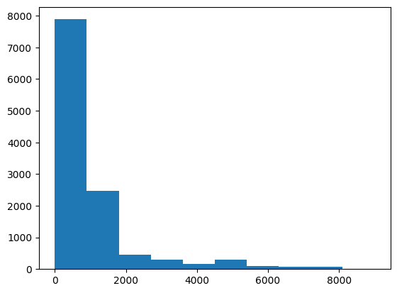
Note the use of the data argument in which we pass a dataframe, exactly as we did with a dictionary in the Matplotlib chapter. Here we filtered protests with more than 10000 participants for visualization purposes.
With hvplot#
If you have hvplot installed, you can also make interactive plots from a dataframe, using the .hvplot accessor:
protests.filter(f).hvplot.scatter(x='start_date', y='participants', by='protester_violence')
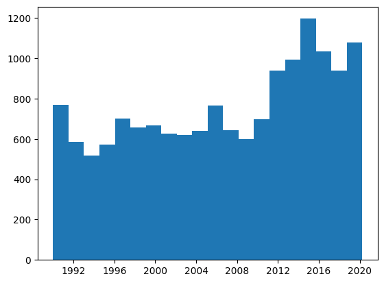
Exercise - time distribution#
Plot the distribution of start_date in the dataset, first with plt, and then with hvplot, using 20 bins in both cases.
Show code cell source
plt.hist('start_date', data=protests, bins=20);
Show code cell source
protests.hvplot.hist('start_date', bins=20)
Note
Method and argument names are not always the same between plt and hvplot, but most of the time, they are!
Aggregate#
Here we’ll cover the very basics of Dataframe aggregation. To go further, you can check out the documentation.
Globally#
There is a number of statistics we can get from our dataset. For instance, we could compute the average duration of protests, as follows:
avg_duration = protests.select(pl.col("duration").mean().alias("average_duration"))
avg_duration
| average_duration |
|---|
| duration[ms] |
| 2d 14h 35m 1s 82ms |
If you want to extract this single value into a usual Python type, you can use the .item() method:
avg_duration.item()
datetime.timedelta(days=2, seconds=52501, microseconds=82000)
See also
For an extensive list of operations that give aggregate results, see the documentation.
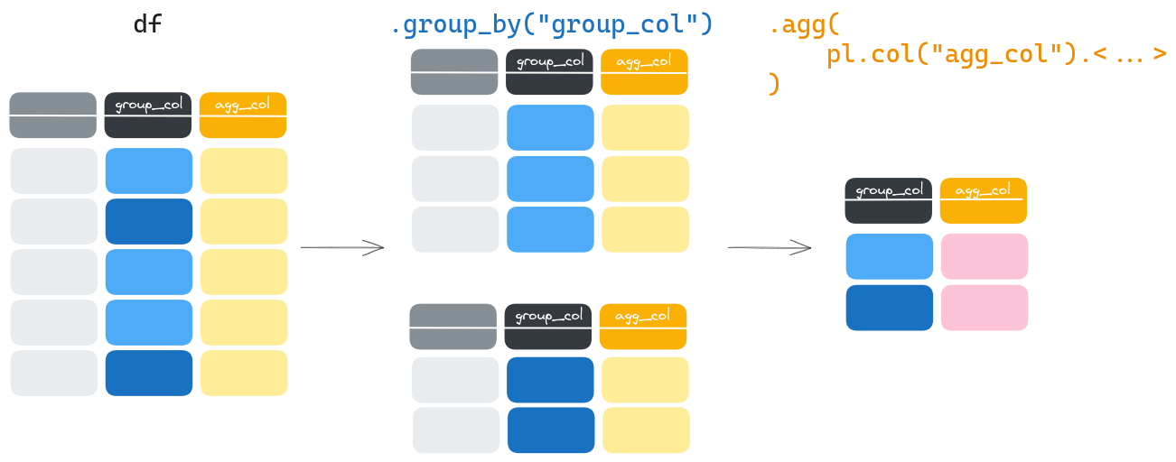
Let’s group by something!#
Now what if we want to get this statistic by country? That’s what the group_by method is made for. To get an idea of what a group is, let us group by country, and look at the very first group as follows:
for (group, df) in protests.group_by('country'):
    print(group)
    display(df)
    break
('Mauritania',)
| id | country | protester_violence | participants | start_date | end_date | duration |
|---|---|---|---|---|---|---|
| i64 | str | bool | i64 | date | date | duration[ms] |
| 4351991001 | "Mauritania" | true | null | 1991-06-02 | 1991-06-02 | 1d |
| 4351991002 | "Mauritania" | false | 150 | 1991-08-12 | 1991-08-12 | 1d |
| 4351992001 | "Mauritania" | false | 1000 | 1992-01-16 | 1992-01-16 | 1d |
| 4351992002 | "Mauritania" | false | 20000 | 1992-01-18 | 1992-01-18 | 1d |
| 4351992003 | "Mauritania" | false | 50 | 1992-01-24 | 1992-01-24 | 1d |
| … | … | … | … | … | … | … |
| 4352016003 | "Mauritania" | true | 50 | 2016-07-04 | 2016-07-04 | 1d |
| 4352016004 | "Mauritania" | false | 50 | 2016-07-11 | 2016-07-11 | 1d |
| 4352016005 | "Mauritania" | false | 100 | 2016-11-15 | 2016-11-15 | 1d |
| 4352016006 | "Mauritania" | true | 1000 | 2016-12-20 | 2016-12-20 | 1d |
| 4352017001 | "Mauritania" | false | 1000 | 2017-01-31 | 2017-01-31 | 1d |
As you can see, when iterating over a group_by result, at each iteration we get a tuple. Its first element is the value of the group_by key (here, the country name), and its second the DataFrame corresponding to this value.
Let’s aggregate#
Now let’s say we want to get the average duration of protests that happened in each country. Naively, you could take the code above and compute the mean at each for iteration. Good news is, there is a simpler, faster way to do it, chaining the .agg() method:
protests.group_by("country").agg(pl.col("duration").mean().alias("average_duration")).head()
| country | average_duration |
|---|---|
| str | duration[ms] |
| "Azerbaijan" | 1d 18h 28m 34s 285ms |
| "Mongolia" | 1d 6h 14m 24s |
| "Yemen" | 1d 19h 6m 29s 808ms |
| "Egypt" | 3d 13h 20m |
| "India" | 6d 6h 26m 57s 621ms |
And, exactly as with .with_columns() or .select(), you may perform as many aggregations as you want.
Try now to also add a new column to the dataframe above, featuring the number of protests by country, and sort the result so that countries with the most protests appear first (refer to the documentation linked above!):
Show code cell content
country_stats = (
    protests.group_by("country")
    .agg(
        pl.col("duration").mean().alias("average_duration"),
        pl.col("id").count().alias("number_of_protests"),
    )
    .sort(by="number_of_protests", descending=True)
)
country_stats
| country | average_duration | number_of_protests |
|---|---|---|
| str | duration[ms] | u32 |
| "United Kingdom" | 1d 23h 55m 1s 38ms | 578 |
| "France" | 2d 7h 24m 53s 967ms | 547 |
| "Ireland" | 1d 1h 10m 9s 744ms | 431 |
| "Germany" | 1d 23h 36m 15s 824ms | 364 |
| "Kenya" | 1d 6h 55m 32s 571ms | 350 |
| … | … | … |
| "Laos" | 1d | 2 |
| "Cape Verde" | 1d | 2 |
| "Bhutan" | 4d | 2 |
| "Qatar" | 6d | 1 |
| "South Sudan" | 2d | 1 |
Exercise - Top protesters#
Make a bar plot showing the number of protests in the 10 countries which had the most protests in their history.
Tip
You can use Axes.barh to make a horizontal bar plot.
Show code cell source
fig, ax = plt.subplots()
ax.barh('country', 'number_of_protests', data=country_stats.head(10).reverse())
ax.set_xlabel('Number of protests');
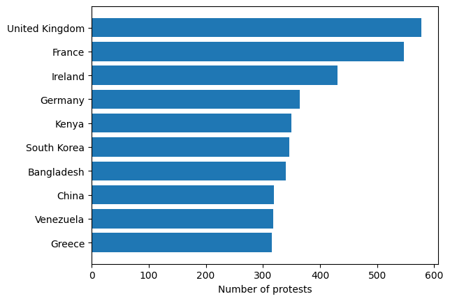
Tip
When you have long categorical labels, such as country names here, it’s often a good idea to use a horizontal bar plot.
Modifying a dataframe by plugging in the result of a grouping#
Sometimes, we may want to compute an aggregate statistic, to then use it to compute a metric in a new column. For instance, it is very common to want to compute a proportion or a ratio, which involves dividing a count by the sum of elements pertaining to each group. Let’s then compute for each protest the ratio of participants that it represented.
If we proceed as above, we’d start by performing the following group_by aggregation:
protests.group_by("country").agg(pl.col("participants").sum().alias("participants_sum")).head()
| country | participants_sum |
|---|---|
| str | i64 |
| "Taiwan" | 7275000 |
| "Croatia" | 290310 |
| "Djibouti" | 4550 |
| "Netherlands" | 2885 |
| "Nepal" | 1014954 |
In fact, in that case we don’t need to call group_by(), but rather:
protests = protests.with_columns(
    pl.col("participants").sum().over("country").alias("participants_sum")
).with_columns(participant_ratio=pl.col("participants") / pl.col("participants_sum"))
protests.head()
| id | country | protester_violence | participants | start_date | end_date | duration | participants_sum | participant_ratio |
|---|---|---|---|---|---|---|---|---|
| i64 | str | bool | i64 | date | date | duration[ms] | i64 | f64 |
| 201990001 | "Canada" | false | 1000 | 1990-01-15 | 1990-01-15 | 1d | 617570 | 0.001619 |
| 201990002 | "Canada" | false | 1000 | 1990-06-25 | 1990-06-25 | 1d | 617570 | 0.001619 |
| 201990003 | "Canada" | false | 500 | 1990-07-01 | 1990-07-01 | 1d | 617570 | 0.00081 |
| 201990004 | "Canada" | true | 100 | 1990-07-12 | 1990-09-06 | 57d | 617570 | 0.000162 |
| 201990005 | "Canada" | true | 950 | 1990-08-14 | 1990-08-15 | 2d | 617570 | 0.001538 |
In the end, all you want to do is add a column, so you start as always by calling .with_columns() and selecting the column from which you’ll use the data with pl.col("participants"). The new element here is that, then, you perform the .sum().over() operation, that will perform the transformation (the sum) over the window defined by the argument of over() (here, the “country” column values).
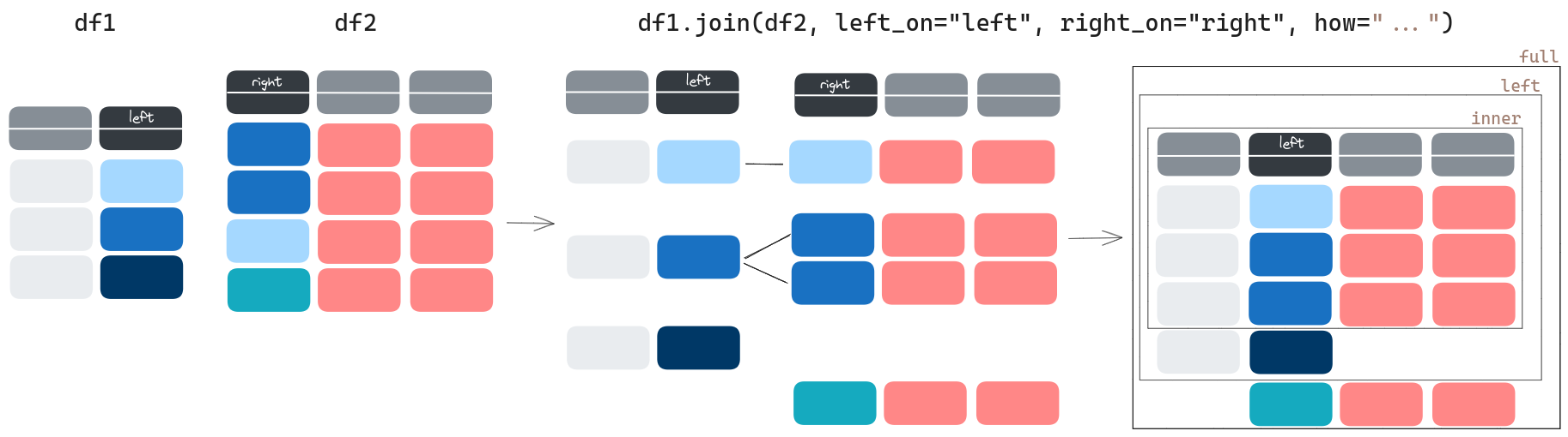
Joining tables#
Suppose we want to add a column to protests with the population of each country, to compute the proportion of the population that participated in each protest, for instance.
To do so, we would need to join our dataset with another one containing such information.
Getting another table#
To get the population of each country, we can take for example the dataset countries_pop.csv, from the World Bank:
countries_pop = pl.read_csv('data/countries_pop.csv')
---------------------------------------------------------------------------
ComputeError                              Traceback (most recent call last)
Cell In[18], line 1
----> 1 countries_pop = pl.read_csv('data/countries_pop.csv')

File /opt/hostedtoolcache/Python/3.11.10/x64/lib/python3.11/site-packages/polars/_utils/deprecation.py:92, in deprecate_renamed_parameter.<locals>.decorate.<locals>.wrapper(*args, **kwargs)
     87 @wraps(function)
     88 def wrapper(*args: P.args, **kwargs: P.kwargs) -> T:
     89     _rename_keyword_argument(
     90         old_name, new_name, kwargs, function.__qualname__, version
     91     )
---> 92     return function(*args, **kwargs)

File /opt/hostedtoolcache/Python/3.11.10/x64/lib/python3.11/site-packages/polars/io/csv/functions.py:508, in read_csv(source, has_header, columns, new_columns, separator, comment_prefix, quote_char, skip_rows, schema, schema_overrides, null_values, missing_utf8_is_empty_string, ignore_errors, try_parse_dates, n_threads, infer_schema, infer_schema_length, batch_size, n_rows, encoding, low_memory, rechunk, use_pyarrow, storage_options, skip_rows_after_header, row_index_name, row_index_offset, sample_size, eol_char, raise_if_empty, truncate_ragged_lines, decimal_comma, glob)
    500 else:
    501     with prepare_file_arg(
    502         source,
    503         encoding=encoding,
   (...)
    506         storage_options=storage_options,
    507     ) as data:
--> 508         df = _read_csv_impl(
    509             data,
    510             has_header=has_header,
    511             columns=columns if columns else projection,
    512             separator=separator,
    513             comment_prefix=comment_prefix,
    514             quote_char=quote_char,
    515             skip_rows=skip_rows,
    516             schema_overrides=schema_overrides,
    517             schema=schema,
    518             null_values=null_values,
    519             missing_utf8_is_empty_string=missing_utf8_is_empty_string,
    520             ignore_errors=ignore_errors,
    521             try_parse_dates=try_parse_dates,
    522             n_threads=n_threads,
    523             infer_schema_length=infer_schema_length,
    524             batch_size=batch_size,
    525             n_rows=n_rows,
    526             encoding=encoding if encoding == "utf8-lossy" else "utf8",
    527             low_memory=low_memory,
    528             rechunk=rechunk,
    529             skip_rows_after_header=skip_rows_after_header,
    530             row_index_name=row_index_name,
    531             row_index_offset=row_index_offset,
    532             eol_char=eol_char,
    533             raise_if_empty=raise_if_empty,
    534             truncate_ragged_lines=truncate_ragged_lines,
    535             decimal_comma=decimal_comma,
    536             glob=glob,
    537         )
    539 if new_columns:
    540     return _update_columns(df, new_columns)

File /opt/hostedtoolcache/Python/3.11.10/x64/lib/python3.11/site-packages/polars/io/csv/functions.py:653, in _read_csv_impl(source, has_header, columns, separator, comment_prefix, quote_char, skip_rows, schema, schema_overrides, null_values, missing_utf8_is_empty_string, ignore_errors, try_parse_dates, n_threads, infer_schema_length, batch_size, n_rows, encoding, low_memory, rechunk, skip_rows_after_header, row_index_name, row_index_offset, sample_size, eol_char, raise_if_empty, truncate_ragged_lines, decimal_comma, glob)
    649         raise ValueError(msg)
    651 projection, columns = parse_columns_arg(columns)
--> 653 pydf = PyDataFrame.read_csv(
    654     source,
    655     infer_schema_length,
    656     batch_size,
    657     has_header,
    658     ignore_errors,
    659     n_rows,
    660     skip_rows,
    661     projection,
    662     separator,
    663     rechunk,
    664     columns,
    665     encoding,
    666     n_threads,
    667     path,
    668     dtype_list,
    669     dtype_slice,
    670     low_memory,
    671     comment_prefix,
    672     quote_char,
    673     processed_null_values,
    674     missing_utf8_is_empty_string,
    675     try_parse_dates,
    676     skip_rows_after_header,
    677     parse_row_index_args(row_index_name, row_index_offset),
    678     eol_char=eol_char,
    679     raise_if_empty=raise_if_empty,
    680     truncate_ragged_lines=truncate_ragged_lines,
    681     decimal_comma=decimal_comma,
    682     schema=schema,
    683 )
    684 return wrap_df(pydf)

ComputeError: found more fields than defined in 'Schema'

Consider setting 'truncate_ragged_lines=True'.
Ah, looks like we’re off to a great start! And that error message is not the clearest. So let’s have a quick look at our data file:
!head data/countries_pop.csv
"Data Source","World Development Indicators",


"Last Updated Date","2024-05-30",


"Country Name","Country Code","Indicator Name","Indicator Code","1960","1961","1962","1963","1964","1965","1966","1967","1968","1969","1970","1971","1972","1973","1974","1975","1976","1977","1978","1979","1980","1981","1982","1983","1984","1985","1986","1987","1988","1989","1990","1991","1992","1993","1994","1995","1996","1997","1998","1999","2000","2001","2002","2003","2004","2005","2006","2007","2008","2009","2010","2011","2012","2013","2014","2015","2016","2017","2018","2019","2020","2021","2022","2023",

"Aruba","ABW","Population, total","SP.POP.TOTL","54608","55811","56682","57475","58178","58782","59291","59522","59471","59330","59106","58816","58855","59365","60028","60715","61193","61465","61738","62006","62267","62614","63116","63683","64174","64478","64553","64450","64332","64596","65712","67864","70192","72360","74710","77050","79417","81858","84355","86867","89101","90691","91781","92701","93540","94483","95606","96787","97996","99212","100341","101288","102112","102880","103594","104257","104874","105439","105962","106442","106585","106537","106445","",

"Africa Eastern and Southern","AFE","Population, total","SP.POP.TOTL","130692579","134169237","137835590","141630546","145605995","149742351","153955516","158313235","162875171","167596160","172475766","177503186","182599092","187901657","193512956","199284304","205202669","211120911","217481420","224315978","230967858","237937461","245386717","252779730","260209149","267938123","276035920","284490394","292795186","301124880","309890664","318544083","326933522","335625136","344418362","353466601","362985802","372352230","381715600","391486231","401600588","412001885","422741118","433807484","445281555","457153837","469508516","482406426","495748900","509410477","523459657","537792950","552530654","567892149","583651101","600008424","616377605","632746570","649757148","667242986","685112979","702977106","720859132","",

"Afghanistan","AFG","Population, total","SP.POP.TOTL","8622466","8790140","8969047","9157465","9355514","9565147","9783147","10010030","10247780","10494489","10752971","11015857","11286753","11575305","11869879","12157386","12425267","12687301","12938862","12986369","12486631","11155195","10088289","9951449","10243686","10512221","10448442","10322758","10383460","10673168","10694796","10745167","12057433","14003760","15455555","16418912","17106595","17788819","18493132","19262847","19542982","19688632","21000256","22645130","23553551","24411191","25442944","25903301","26427199","27385307","28189672","29249157","30466479","31541209","32716210","33753499","34636207","35643418","36686784","37769499","38972230","40099462","41128771","",

"Africa Western and Central","AFW","Population, total","SP.POP.TOTL","97256290","99314028","101445032","103667517","105959979","108336203","110798486","113319950","115921723","118615741","121424797","124336039","127364044","130563107","133953892","137548613","141258400","145122851","149206663","153459665","157825609","162323313","167023385","171566640","176054495","180817312","185720244","190759952","195969722","201392200","206739024","212172888","217966101","223788766","229675775","235861484","242200260","248713095","255482918","262397030","269611898","277160097","284952322","292977949","301265247","309824829","318601484","327612838","336893835","346475221","356337762","366489204","376797999","387204553","397855507","408690375","419778384","431138704","442646825","454306063","466189102","478185907","490330870","",

"Angola","AGO","Population, total","SP.POP.TOTL","5357195","5441333","5521400","5599827","5673199","5736582","5787044","5827503","5868203","5928386","6029700","6177049","6364731","6578230","6802494","7032713","7266780","7511895","7771590","8043218","8330047","8631457","8947152","9276707","9617702","9970621","10332574","10694057","11060261","11439498","11828638","12228691","12632507","13038270","13462031","13912253","14383350","14871146","15366864","15870753","16394062","16941587","17516139","18124342","18771125","19450959","20162340","20909684","21691522","22507674","23364185","24259111","25188292","26147002","27128337","28127721","29154746","30208628","31273533","32353588","33428486","34503774","35588987","",
Note
Here, we use the cell magic ! to run a system command called head, which, exactly as for dataframes (or is it the other way around?), shows you the first lines of a file. You’re not expected to learn this kind of commands in this course, this was simply to show that you can do that in Jupyter, and that it’s very practical.
Question
Having seen that, can you guess what the problem was? How is this file different from the ones we’ve seen previously?
Answer
The 4 first lines actually contain some metadata about the file, and the header specifying column names is only on the 5th line! That’s why Polars complains about the Schema, it thought that the first line was defining the columns, but then found more columns in following lines. Fortunately, Polars lets us skip rows from CSV files, using the skip_rows argument.
countries_pop = pl.read_csv('data/countries_pop.csv', skip_rows=4)
countries_pop.head()
| Country Name | Country Code | Indicator Name | Indicator Code | 1960 | 1961 | 1962 | 1963 | 1964 | 1965 | 1966 | 1967 | 1968 | 1969 | 1970 | 1971 | 1972 | 1973 | 1974 | 1975 | 1976 | 1977 | 1978 | 1979 | 1980 | 1981 | 1982 | 1983 | 1984 | 1985 | 1986 | 1987 | 1988 | 1989 | 1990 | 1991 | 1992 | 1993 | 1994 | 1995 | 1996 | 1997 | 1998 | 1999 | 2000 | 2001 | 2002 | 2003 | 2004 | 2005 | 2006 | 2007 | 2008 | 2009 | 2010 | 2011 | 2012 | 2013 | 2014 | 2015 | 2016 | 2017 | 2018 | 2019 | 2020 | 2021 | 2022 | 2023 | |
|---|---|---|---|---|---|---|---|---|---|---|---|---|---|---|---|---|---|---|---|---|---|---|---|---|---|---|---|---|---|---|---|---|---|---|---|---|---|---|---|---|---|---|---|---|---|---|---|---|---|---|---|---|---|---|---|---|---|---|---|---|---|---|---|---|---|---|---|---|
| str | str | str | str | i64 | i64 | i64 | i64 | i64 | i64 | i64 | i64 | i64 | i64 | i64 | i64 | i64 | i64 | i64 | i64 | i64 | i64 | i64 | i64 | i64 | i64 | i64 | i64 | i64 | i64 | i64 | i64 | i64 | i64 | i64 | i64 | i64 | i64 | i64 | i64 | i64 | i64 | i64 | i64 | i64 | i64 | i64 | i64 | i64 | i64 | i64 | i64 | i64 | i64 | i64 | i64 | i64 | i64 | i64 | i64 | i64 | i64 | i64 | i64 | i64 | i64 | i64 | str | str |
| "Aruba" | "ABW" | "Population, total" | "SP.POP.TOTL" | 54608 | 55811 | 56682 | 57475 | 58178 | 58782 | 59291 | 59522 | 59471 | 59330 | 59106 | 58816 | 58855 | 59365 | 60028 | 60715 | 61193 | 61465 | 61738 | 62006 | 62267 | 62614 | 63116 | 63683 | 64174 | 64478 | 64553 | 64450 | 64332 | 64596 | 65712 | 67864 | 70192 | 72360 | 74710 | 77050 | 79417 | 81858 | 84355 | 86867 | 89101 | 90691 | 91781 | 92701 | 93540 | 94483 | 95606 | 96787 | 97996 | 99212 | 100341 | 101288 | 102112 | 102880 | 103594 | 104257 | 104874 | 105439 | 105962 | 106442 | 106585 | 106537 | 106445 | "" | null |
| "Africa Eastern and Southern" | "AFE" | "Population, total" | "SP.POP.TOTL" | 130692579 | 134169237 | 137835590 | 141630546 | 145605995 | 149742351 | 153955516 | 158313235 | 162875171 | 167596160 | 172475766 | 177503186 | 182599092 | 187901657 | 193512956 | 199284304 | 205202669 | 211120911 | 217481420 | 224315978 | 230967858 | 237937461 | 245386717 | 252779730 | 260209149 | 267938123 | 276035920 | 284490394 | 292795186 | 301124880 | 309890664 | 318544083 | 326933522 | 335625136 | 344418362 | 353466601 | 362985802 | 372352230 | 381715600 | 391486231 | 401600588 | 412001885 | 422741118 | 433807484 | 445281555 | 457153837 | 469508516 | 482406426 | 495748900 | 509410477 | 523459657 | 537792950 | 552530654 | 567892149 | 583651101 | 600008424 | 616377605 | 632746570 | 649757148 | 667242986 | 685112979 | 702977106 | 720859132 | "" | null |
| "Afghanistan" | "AFG" | "Population, total" | "SP.POP.TOTL" | 8622466 | 8790140 | 8969047 | 9157465 | 9355514 | 9565147 | 9783147 | 10010030 | 10247780 | 10494489 | 10752971 | 11015857 | 11286753 | 11575305 | 11869879 | 12157386 | 12425267 | 12687301 | 12938862 | 12986369 | 12486631 | 11155195 | 10088289 | 9951449 | 10243686 | 10512221 | 10448442 | 10322758 | 10383460 | 10673168 | 10694796 | 10745167 | 12057433 | 14003760 | 15455555 | 16418912 | 17106595 | 17788819 | 18493132 | 19262847 | 19542982 | 19688632 | 21000256 | 22645130 | 23553551 | 24411191 | 25442944 | 25903301 | 26427199 | 27385307 | 28189672 | 29249157 | 30466479 | 31541209 | 32716210 | 33753499 | 34636207 | 35643418 | 36686784 | 37769499 | 38972230 | 40099462 | 41128771 | "" | null |
| "Africa Western and Central" | "AFW" | "Population, total" | "SP.POP.TOTL" | 97256290 | 99314028 | 101445032 | 103667517 | 105959979 | 108336203 | 110798486 | 113319950 | 115921723 | 118615741 | 121424797 | 124336039 | 127364044 | 130563107 | 133953892 | 137548613 | 141258400 | 145122851 | 149206663 | 153459665 | 157825609 | 162323313 | 167023385 | 171566640 | 176054495 | 180817312 | 185720244 | 190759952 | 195969722 | 201392200 | 206739024 | 212172888 | 217966101 | 223788766 | 229675775 | 235861484 | 242200260 | 248713095 | 255482918 | 262397030 | 269611898 | 277160097 | 284952322 | 292977949 | 301265247 | 309824829 | 318601484 | 327612838 | 336893835 | 346475221 | 356337762 | 366489204 | 376797999 | 387204553 | 397855507 | 408690375 | 419778384 | 431138704 | 442646825 | 454306063 | 466189102 | 478185907 | 490330870 | "" | null |
| "Angola" | "AGO" | "Population, total" | "SP.POP.TOTL" | 5357195 | 5441333 | 5521400 | 5599827 | 5673199 | 5736582 | 5787044 | 5827503 | 5868203 | 5928386 | 6029700 | 6177049 | 6364731 | 6578230 | 6802494 | 7032713 | 7266780 | 7511895 | 7771590 | 8043218 | 8330047 | 8631457 | 8947152 | 9276707 | 9617702 | 9970621 | 10332574 | 10694057 | 11060261 | 11439498 | 11828638 | 12228691 | 12632507 | 13038270 | 13462031 | 13912253 | 14383350 | 14871146 | 15366864 | 15870753 | 16394062 | 16941587 | 17516139 | 18124342 | 18771125 | 19450959 | 20162340 | 20909684 | 21691522 | 22507674 | 23364185 | 24259111 | 25188292 | 26147002 | 27128337 | 28127721 | 29154746 | 30208628 | 31273533 | 32353588 | 33428486 | 34503774 | 35588987 | "" | null |
As you can see, there is one row per country, and the population counts are given in separate columns, for years ranging between 1960 and 2022. So in principle, when adding in the population data to protests, we should add the population corresponding to the protest’s year. For the sake of simplicity though, here we’ll take populations from a single year. But let’s at least choose it reasonably. We’ve already seen graphically the distribution of start_date, but let’s get some summary statistics.
As a small exercise, try to get the following table (hint: use the Dataframe.describe() method):
Show code cell source
protests.select(pl.col('start_date')).describe()
| statistic | start_date |
|---|---|
| str | str |
| "count" | "15239" |
| "null_count" | "0" |
| "mean" | "2006-10-19 22:55:04.941000" |
| "std" | null |
| "min" | "1990-01-01" |
| "25%" | "1999-02-08" |
| "50%" | "2007-10-25" |
| "75%" | "2014-11-15" |
| "max" | "2020-03-31" |
We see that the average sits toward the end of 2006, while the median towards the end of 2007. Let us then take 2007 as our year to get populations. Go ahead and assign a new variable countries_single_pop with the dataframe containing the populations of that year:
Show code cell source
countries_single_pop = countries_pop.select(
    pl.col("Country Name").alias("country"),
    pl.col("2007").alias("pop_2007"),
)
countries_single_pop.head()
| country | pop_2007 |
|---|---|
| str | i64 |
| "Aruba" | 96787 |
| "Africa Eastern and Southern" | 482406426 |
| "Afghanistan" | 25903301 |
| "Africa Western and Central" | 327612838 |
| "Angola" | 20909684 |
Performing the join#
Now, adding in these populations to protests is as simple as:
protests_with_pop = protests.join(countries_single_pop, on="country")
protests_with_pop.head()
| id | country | protester_violence | participants | start_date | end_date | duration | participants_sum | participant_ratio | pop_2007 |
|---|---|---|---|---|---|---|---|---|---|
| i64 | str | bool | i64 | date | date | duration[ms] | i64 | f64 | i64 |
| 201990001 | "Canada" | false | 1000 | 1990-01-15 | 1990-01-15 | 1d | 617570 | 0.001619 | 32889025 |
| 201990002 | "Canada" | false | 1000 | 1990-06-25 | 1990-06-25 | 1d | 617570 | 0.001619 | 32889025 |
| 201990003 | "Canada" | false | 500 | 1990-07-01 | 1990-07-01 | 1d | 617570 | 0.00081 | 32889025 |
| 201990004 | "Canada" | true | 100 | 1990-07-12 | 1990-09-06 | 57d | 617570 | 0.000162 | 32889025 |
| 201990005 | "Canada" | true | 950 | 1990-08-14 | 1990-08-15 | 2d | 617570 | 0.001538 | 32889025 |
The on argument allows you to set the column the join will consider to match. Here, the column "country" exists in both Dataframes, so we can simply set it to that. However, if, for instance, countries_single_pop still had the "Country Name" column, instead of on="country", we’d have had to specify left_on="country", right_on="Country Name".
join has another very important argument: how. To get an idea of what it does, let us compare the shape of protests_with_pop with the original protests:
protests_with_pop.shape, protests.shape
((12743, 10), (15239, 9))
As you can see, we lost some rows! Why? Because by default, the argument how is set to "inner". This means that the dataframe output by join will only have rows for which the "country" exists in both input dataframes. To conserve the rows of the original dataframe, you can set how="left" instead:
full_protests_with_pop = protests.join(countries_single_pop, on="country", how="left")
full_protests_with_pop.shape
(15239, 10)
And we did conserve our number of rows.
Question
But then, what happened to rows in which we could not find a matching country in countries_single_pop?
Answer
They have null values in "pop_2007", to represent an absence of data. Try to get the rows for which this is the case.
Exercise - proportion of protesters#
Compute the proportion of the total population that protested in each protest, and show the countries in which the maximum proportion is highest.
Show code cell source
top_protesters = (
    protests_with_pop.with_columns(
        prop_of_pop=pl.col("participants") / pl.col("pop_2007")
    )
    .group_by("country")
    .agg(pl.col("prop_of_pop").max().alias("max_prop_of_pop"))
    .sort(by="max_prop_of_pop", descending=True, nulls_last=True)
)
top_protesters.head()
| country | max_prop_of_pop |
|---|---|
| str | f64 |
| "Lebanon" | 0.207917 |
| "Moldova" | 0.139164 |
| "Armenia" | 0.133138 |
| "Guinea" | 0.104744 |
| "Greece" | 0.09051 |
Now slightly harder, try to get the full row corresponding to that protest in which the maximum "prop_of_pop" was reached.
Hint
You’ll find the Expression.sort_by() method useful for that.
Show code cell source
top_protesters = (
    protests_with_pop.with_columns(
        prop_of_pop=pl.col("participants") / pl.col("pop_2007")
    )
    .group_by("country")
    .agg(pl.all().sort_by("prop_of_pop").last())
    .sort(by="prop_of_pop", descending=True, nulls_last=True)
)
top_protesters.head()
| country | id | protester_violence | participants | start_date | end_date | duration | participants_sum | participant_ratio | pop_2007 | prop_of_pop |
|---|---|---|---|---|---|---|---|---|---|---|
| str | i64 | bool | i64 | date | date | duration[ms] | i64 | f64 | i64 | f64 |
| "Lebanon" | 6602006001 | false | 1000000 | 2006-02-15 | 2006-02-15 | 1d | 4800000 | 0.208333 | 4809608 | 0.207917 |
| "Moldova" | 3591991003 | false | 400000 | 1991-08-21 | 1991-08-21 | 1d | 1112256 | 0.359629 | 2874299 | 0.139164 |
| "Armenia" | 3711992001 | false | 400000 | 1992-11-02 | 1992-11-02 | 1d | 1616170 | 0.247499 | 3004393 | 0.133138 |
| "Guinea" | 4382019010 | false | 1000000 | 2019-12-10 | 2019-12-10 | 1d | 2647050 | 0.377779 | 9547082 | 0.104744 |
| "Greece" | 3502012001 | true | 1000000 | 2012-02-07 | 2012-02-07 | 1d | 3302570 | 0.302794 | 11048473 | 0.09051 |
Exercise - doing things right#
Beforehand, we just took the population of a single year, while each protest happened on different years. In reality, we can know this year from the "start_date" column. Reproduce the above to get protests_with_pop, taking into account the right population.
Tip
To start off, you’ll need to call the Dataframe method
.unpivot()oncountries_pop.To select all year columns, don’t write them by hand! There are (at least) two ways to select all of them lazily.
Show code cell source
import polars.selectors as cs

countries_actual_pop = (
    countries_pop.select(pl.col("Country Name").alias("country"), cs.by_dtype(pl.Int64))
    .unpivot(index="country", variable_name="year", value_name="pop")
    .with_columns(pl.col("year").cast(pl.Int32))
)
protests_with_pop = protests.with_columns(pl.col('start_date').dt.year().alias("year")).join(countries_actual_pop, on=['country', "year"])
protests_with_pop.head()
| id | country | protester_violence | participants | start_date | end_date | duration | participants_sum | participant_ratio | year | pop |
|---|---|---|---|---|---|---|---|---|---|---|
| i64 | str | bool | i64 | date | date | duration[ms] | i64 | f64 | i32 | i64 |
| 3391990001 | "Albania" | false | null | 1990-07-06 | 1990-07-06 | 1d | 381150 | null | 1990 | 3286542 |
| 3391990002 | "Albania" | true | null | 1990-12-09 | 1990-12-09 | 1d | 381150 | null | 1990 | 3286542 |
| 3391990003 | "Albania" | false | 9000 | 1990-12-12 | 1990-12-12 | 1d | 381150 | 0.023613 | 1990 | 3286542 |
| 3391990004 | "Albania" | true | 50 | 1990-12-13 | 1990-12-13 | 1d | 381150 | 0.000131 | 1990 | 3286542 |
| 3391990005 | "Albania" | true | null | 1990-12-15 | 1990-12-16 | 2d | 381150 | null | 1990 | 3286542 |
Now, check that it worked by checking out Italy, for instance.
Show code cell source
yearly_pop_italy = protests_with_pop.filter(pl.col('country') == 'Italy').select('year', 'pop').group_by('year').agg(pl.all().first()).sort('year')
yearly_pop_italy
| year | pop |
|---|---|
| i32 | i64 |
| 1990 | 56719240 |
| 1991 | 56758521 |
| 1992 | 56797087 |
| 1993 | 56831821 |
| 1994 | 56843400 |
| … | … |
| 2014 | 60789140 |
| 2016 | 60627498 |
| 2017 | 60536709 |
| 2018 | 60421760 |
| 2019 | 59729081 |
Be lazy#
A great strength of Polars is its lazy mode. In this mode, instead of working with Dataframes, you work with Lazyframes. The big difference between the two is that, while Dataframes actually hold data, Lazyframes just hold a set of operations to execute.
Working with a Lazyframe#
The first way to obtain a Lazyframe is to call the .lazy() method on an existing Dataframe, like so:
type(protests.lazy())
polars.lazyframe.frame.LazyFrame
But actually, to get the most out of the lazy mode, you should rather work with Lazyframes before you even read any data. In practice, this means that, instead of calling pl.read_<file-format>() to read from a data source, you’ll call an equivalent pl.scan_<file-format>(). For instance:
lazy_protests = pl.scan_csv('data/protests.csv')
lazy_protests
NAIVE QUERY PLAN
run LazyFrame.show_graph() to see the optimized version
As you can see, no data is shown, simply because no data was read! With this object, you can now call all methods seen until now, as if you were dealing with a regular Dataframe. In order to actually get the result of a computation, you simply need to call the .collect() method at the very end.
Let us show by example the power of using Lazyframes. Let’s compute the median number of participants by year in Italy, in a particularly stupid way:
%%time
dumb_agg = (
    pl.read_csv("data/protests.csv")
    .with_columns(
        pl.col("participants").str.extract("([0-9]+)").cast(int),
    )
    .group_by("country", "year")
    .agg(pl.col("participants").median())
    .filter(pl.col("country") == "Italy")
)
dumb_agg.head()
CPU times: user 45.1 ms, sys: 9.56 ms, total: 54.7 ms
Wall time: 17 ms
| country | year | participants |
|---|---|---|
| str | i64 | f64 |
| "Italy" | 1993 | 50000.0 |
| "Italy" | 1994 | 500025.0 |
| "Italy" | 2018 | 75.0 |
| "Italy" | 2005 | 1200.0 |
| "Italy" | 1998 | 575.0 |
Question
Why is this not very smart? How could we make this operation more efficient?
Answer
Because we’re computing this median for every single country, while we’re only interested in Italy here! The filter() should be called directly after reading the CSV.
Let’s time the same thing, except that we do everything in lazy mode:
%%time
lazy_agg = (
    pl.scan_csv("data/protests.csv")
    .with_columns(
        pl.col("participants").str.extract("([0-9]+)").cast(int),
    )
    .group_by("country", "year")
    .agg(pl.col("participants").median())
    .filter(pl.col("country") == "Italy")
)
lazy_agg.collect().head()
CPU times: user 10.3 ms, sys: 5.94 ms, total: 16.3 ms
Wall time: 5.05 ms
| country | year | participants |
|---|---|---|
| str | i64 | f64 |
| "Italy" | 2004 | 100.0 |
| "Italy" | 1993 | 50000.0 |
| "Italy" | 1990 | 50.0 |
| "Italy" | 2020 | null |
| "Italy" | 2007 | 10000.0 |
That’s a big difference in timing, and for relatively simple operations performed on a relatively small dataset!
But why is there this difference? It’s because, before calling .collect(), Polars will run what is called a query optimization, and automatically reorder and modify the operations performed in the collect, to make them as optimal as it can. To see that, you can call .show_graph() to find out what the optimization did:
lazy_agg.show_graph()

This is to be read from the bottom up. As you can see, the filter has been pushed down to the very moment data is read! Which does make a lot of sense, doesn’t it?
To sum up, there are two main advantages of using Lazyframes:
You get an automatic query optimization. So even if the code you wrote could be much more optimal, it will run as fast as it can. In other words, being lazy allows you to be dumb and not suffer the consequences.
As filters can be pushed down to the very moment data is read, you don’t need to load all data in memory. This means that you could analyse data files which are too big to fit in your computer memory!
Exercise - Healthcare facilities#
✪✪ Let’s examine the dataset SANSTRUT001.csv which contains the healthcare facilities of Trentino region, and for each tells the type of assistance it offers (clinical activity, diagnostics, etc), the code and name of the communality where it is located.
Data source: dati.trentino.it
License: Creative Commons Attribution 4.0
Write a function strutsan which takes as input a town code and a text string, opens the file lazily and:
Prints also the number of found rows
Returns a dataframe with selected only the rows having that town code and which contain the string in the column
ASSISTENZA. The returned dataset must have only the columnsSTRUTTURA,ASSISTENZA,COD_COMUNE,COMUNE.
Show code cell source
def strutsan(cod_comune, assistenza):
    struprotests = pl.scan_csv("data/SANSTRUT001.csv")
    res = struprotests.filter(
        (pl.col("COD_COMUNE") == cod_comune)
        & pl.col("ASSISTENZA").str.contains(assistenza)
    ).collect()

    print("Found", res.shape[0], "facilities")
    return res.select("STRUTTURA", "ASSISTENZA", "COD_COMUNE", "COMUNE")
strutsan(22050, '') # no ASSISTENZA filter
Found 6 facilities
| STRUTTURA | ASSISTENZA | COD_COMUNE | COMUNE |
|---|---|---|---|
| str | str | i64 | str |
| "PRESIDIO OSPEDALIERO DI CAVALE… | "ATTIVITA` CLINICA" | 22050 | "CAVALESE" |
| "PRESIDIO OSPEDALIERO DI CAVALE… | "DIAGNOSTICA STRUMENTALE E PER … | 22050 | "CAVALESE" |
| "PRESIDIO OSPEDALIERO DI CAVALE… | "ATTIVITA` DI LABORATORIO" | 22050 | "CAVALESE" |
| "CENTRO SALUTE MENTALE CAVALESE" | "ASSISTENZA PSICHIATRICA" | 22050 | "CAVALESE" |
| "CENTRO DIALISI CAVALESE" | "ATTIVITA` CLINICA" | 22050 | "CAVALESE" |
| "CONSULTORIO CAVALESE" | "ATTIVITA` DI CONSULTORIO MATER… | 22050 | "CAVALESE" |
strutsan(22205, 'CLINICA')
Found 16 facilities
| STRUTTURA | ASSISTENZA | COD_COMUNE | COMUNE |
|---|---|---|---|
| str | str | i64 | str |
| "PRESIDIO OSPEDALIERO S.CHIARA" | "ATTIVITA` CLINICA" | 22205 | "TRENTO" |
| "CENTRO DIALISI TRENTO" | "ATTIVITA` CLINICA" | 22205 | "TRENTO" |
| "POLIAMBULATORI S.CHIARA" | "ATTIVITA` CLINICA" | 22205 | "TRENTO" |
| "PRESIDIO OSPEDALIERO VILLA IGE… | "ATTIVITA` CLINICA" | 22205 | "TRENTO" |
| "OSPEDALE CLASSIFICATO S.CAMIL… | "ATTIVITA` CLINICA" | 22205 | "TRENTO" |
| … | … | … | … |
| "COOPERATIVA SOCIALE IRIFOR DEL… | "ATTIVITA` CLINICA" | 22205 | "TRENTO" |
| "AGSAT ASSOCIAZIONE GENITORI SO… | "ATTIVITA` CLINICA" | 22205 | "TRENTO" |
| "AZIENDA PUBBLICA SERVIZI ALLA … | "ATTIVITA` CLINICA" | 22205 | "TRENTO" |
| "CST TRENTO" | "ATTIVITA` CLINICA" | 22205 | "TRENTO" |
| "A.P.S.P. 'BEATO DE TSCHIDERER'… | "ATTIVITA` CLINICA" | 22205 | "TRENTO" |
strutsan(22205, 'LABORATORIO')
Found 5 facilities
| STRUTTURA | ASSISTENZA | COD_COMUNE | COMUNE |
|---|---|---|---|
| str | str | i64 | str |
| "PRESIDIO OSPEDALIERO S.CHIARA" | "ATTIVITA` DI LABORATORIO" | 22205 | "TRENTO" |
| "LABORATORI ADIGE SRL" | "ATTIVITA` DI LABORATORIO" | 22205 | "TRENTO" |
| "LABORATORIO DRUSO SRL" | "ATTIVITA` DI LABORATORIO" | 22205 | "TRENTO" |
| "CASA DI CURA VILLA BIANCA SPA" | "ATTIVITA` DI LABORATORIO" | 22205 | "TRENTO" |
| "CENTRO SERVIZI SANITARI" | "ATTIVITA` DI LABORATORIO" | 22205 | "TRENTO" |
Some more exercises#
Exercise - Air pollutants#
Let’s try to analyse the hourly data from air quality monitoring stations from Autonomous Province of Trento.
Source: dati.trentino.it
Load the file#
✪ Load the file aria.csv in Polars
IMPORTANT 1: put the dataframe into the variable aria, so not to confuse it with the previous datasets.
IMPORTANT 2: use encoding 'latin-1'
(otherwise you might get weird load errors according to your operating system)
Show code cell source
aria = pl.read_csv(
    "data/aria.csv", encoding="latin-1", schema_overrides={"Valore": pl.Float64}
)
aria.head()
| Stazione | Inquinante | Data | Ora | Valore | Unità di misura |
|---|---|---|---|---|---|
| str | str | str | i64 | f64 | str |
| "Parco S. Chiara" | "PM10" | "2019-05-04" | 1 | 17.0 | "µg/mc" |
| "Parco S. Chiara" | "PM10" | "2019-05-04" | 2 | 19.0 | "µg/mc" |
| "Parco S. Chiara" | "PM10" | "2019-05-04" | 3 | 17.0 | "µg/mc" |
| "Parco S. Chiara" | "PM10" | "2019-05-04" | 4 | 15.0 | "µg/mc" |
| "Parco S. Chiara" | "PM10" | "2019-05-04" | 5 | 13.0 | "µg/mc" |
Tip
If you get an error, read it carefully, what is the issue here? What column is causing it? Then, use pl.read_csv? or head over to the documentation and read the Notes, that will get you closer to the solution.
Pollutants average#
✪ find the average of PM10 pollutants at Parco S. Chiara (average on all days).
Show code cell source
aria.filter(
    (pl.col("Stazione") == "Parco S. Chiara") & (pl.col("Inquinante") == "PM10")
).select(pl.col("Valore").mean())
| Valore |
|---|
| f64 |
| 11.385753 |
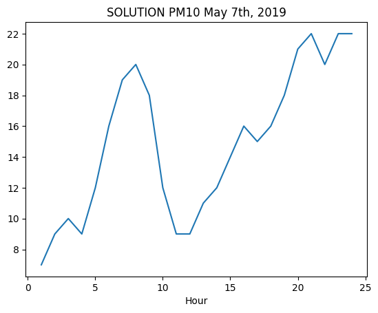
PM10 chart#
✪ Use Axes.plot to show in a chart the values of PM10 in Parco S. Chiara on May 7th, 2019.
Show code cell source
import matplotlib.pyplot as plt

filtered = aria.filter(
    (pl.col("Stazione") == "Parco S. Chiara")
    & (pl.col("Inquinante") == "PM10")
    & (pl.col("Data") == "2019-05-07")
)

fig, ax = plt.subplots()
ax.plot("Ora", "Valore", data=filtered)
ax.set_title("SOLUTION PM10 May 7th, 2019")
ax.set_xlabel("Hour");
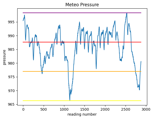
Exercise - meteo pressure intervals#
✪✪✪ The dataset meteo.csv contains the weather data of Trento, November 2017 (source: www.meteotrentino.it). We would like to subdivide the pressure readings into three intervals A (low), B (medium), C (high), and count how many readings have been made for each interval.
IMPORTANT: assign the dataframe to a variable called meteo so to avoid confusion with other dataframes
Where are the intervals?#
First, let’s find the pressure values for these 3 intervals and plot them as segments, so to end up with a chart like this:
Before doing the plot, we will need to know at which height we should plot the segments.
Load the dataset with polars, calculate the following variables and PRINT them
round values with
roundfunctionthe excursion is the difference between minimum and maximum
note
intervalCcoincides with the maximum
DO NOT use min and max as variable names (they are reserved functions!!)
Show code cell source
meteo = pl.read_csv("data/meteo.csv")
minimum = meteo.select("Pressure").min().item()
maximum = meteo.select("Pressure").max().item()
excursion = maximum - minimum
intervalA, intervalB, intervalC = (
    minimum + excursion / 3.0,
    minimum + excursion * 2.0 / 3.0,
    minimum + excursion,
)
intervalA, intervalB, intervalC = (
    round(intervalA, 2),
    round(intervalB, 2),
    round(intervalC, 2),
)

print("minimum:", minimum)
print("maximum:", maximum)
print("excursion:", excursion)
print("intervalA:", intervalA)
print("intervalB:", intervalB)
print("intervalC:", intervalC)
minimum: 966.3
maximum: 998.3
excursion: 32.0
intervalA: 976.97
intervalB: 987.63
intervalC: 998.3
Segments plot#
Try now to plot the chart of pressure and the 4 horizontal segments.
to overlay the segments with different colors, just make repeated calls to
ax.plota segment is defined by two points: so just find the coordinates of those two points..
REMEMBER title and labels
Show code cell source
fig, ax = plt.subplots()
ax.plot("Pressure", data=meteo)
ax.plot([0, meteo.shape[0]], [minimum, minimum], color="yellow")
ax.plot([0, meteo.shape[0]], [intervalA, intervalA], color="orange")
ax.plot([0, meteo.shape[0]], [intervalB, intervalB], color="red")
ax.plot([0, meteo.shape[0]], [intervalC, intervalC], color="purple")
ax.set_title("Meteo Pressure")
ax.set_xlabel("reading number")
ax.set_ylabel("pressure");
Assigning the intervals#
We literally made a picture of where the intervals are located - let’s now ask ourselves how many readings have been done for each interval.
First, try creating a column which assigns to each reading the interval where it belongs to.
Tip
You will need the function pl.when(), start by inspecting it!
Show code cell source
meteo = meteo.with_columns(
    PressureInterval=pl.when(pl.col("Pressure") < intervalA)
    .then(pl.lit("A (low)"))
    .when(pl.col("Pressure") < intervalB)
    .then(pl.lit("B medium"))
    .otherwise(pl.lit("C (high)"))
)
meteo.head()
| Date | Pressure | Rain | Temp | PressureInterval |
|---|---|---|---|---|
| str | f64 | f64 | f64 | str |
| "01/11/2017 00:00" | 995.4 | 0.0 | 5.4 | "C (high)" |
| "01/11/2017 00:15" | 995.5 | 0.0 | 6.0 | "C (high)" |
| "01/11/2017 00:30" | 995.5 | 0.0 | 5.9 | "C (high)" |
| "01/11/2017 00:45" | 995.7 | 0.0 | 5.4 | "C (high)" |
| "01/11/2017 01:00" | 995.7 | 0.0 | 5.3 | "C (high)" |
Grouping by intervals#
a. First, create a grouping to count occurrences:
Show code cell source
press_groups = meteo.group_by("PressureInterval").agg(pl.col("Pressure").count())
press_groups
| PressureInterval | Pressure |
|---|---|
| str | u32 |
| "C (high)" | 1380 |
| "B medium" | 1243 |
| "A (low)" | 255 |
b. Now plot it
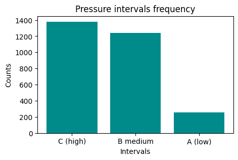
REMEMBER title and axis labels
Show code cell source
fig, ax = plt.subplots(figsize=(5, 3))
ax.bar("PressureInterval", "Pressure", data=press_groups, color="darkcyan")
ax.set_title("Pressure intervals frequency")
ax.set_xlabel("Intervals")
ax.set_ylabel("Counts")
Text(0, 0.5, 'Counts')
Exercise - meteo average temperature#
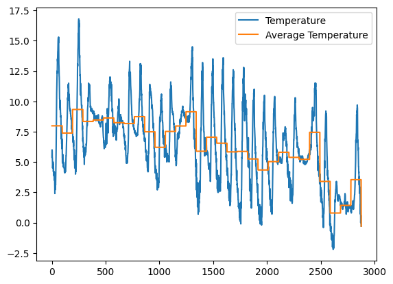
✪✪✪ Calculate the average temperature for each day, and show it in the plot.
HINT: add 'Day' column by extracting only the day from the date. To do it, use the function .str.slice.
Show code cell source
meteo = (
    pl.read_csv("data/meteo.csv")
    .with_columns(pl.col("Date").str.slice(0, 10).alias("Day"))
    .with_columns(pl.col("Temp").mean().over("Day").alias("avg_day_temp"))
)
meteo.head()
| Date | Pressure | Rain | Temp | Day | avg_day_temp |
|---|---|---|---|---|---|
| str | f64 | f64 | f64 | str | f64 |
| "01/11/2017 00:00" | 995.4 | 0.0 | 5.4 | "01/11/2017" | 7.983333 |
| "01/11/2017 00:15" | 995.5 | 0.0 | 6.0 | "01/11/2017" | 7.983333 |
| "01/11/2017 00:30" | 995.5 | 0.0 | 5.9 | "01/11/2017" | 7.983333 |
| "01/11/2017 00:45" | 995.7 | 0.0 | 5.4 | "01/11/2017" | 7.983333 |
| "01/11/2017 01:00" | 995.7 | 0.0 | 5.3 | "01/11/2017" | 7.983333 |
Show code cell source
fig, ax = plt.subplots()
ax.plot("Temp", data=meteo, label="Temperature")
ax.plot("avg_day_temp", data=meteo, label="Average Temperature")
ax.legend();